The Neuron
The neuron is the most basic building bock of an artificial network. The most basic representation of a neural network is shown below.
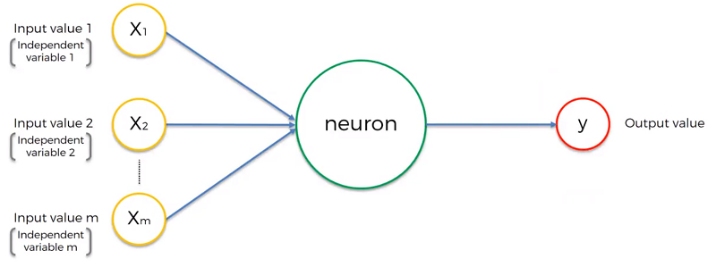
The input values are essentially data (our independent variables). This data is either standardized (has a mean of zero and a variance of one) or sometimes normalize them (minimum value divided by the difference between the minimum and maximum value, for a number between 0 to 1). All these independent values in the end should be in the same range as the neuron will treat them all in a similar fashion.
Additional Read: Efficient BackProp By Yann LeCunn
The Output Value can be:
- Continuous (Like price or a probability)
- Binary
- Categorical (in which case you would want many output value neurons)
The synapses are all assigned separate weights. Weights are essentially an indicator for the neuron in telling it how important the input data it’s getting from it is. These get adjusted by the neural network and is how the network is trained.
The neuron itself does the following:
- Weighted sum of all input values
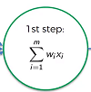
- Apply activation function to the weighted sum.

- Neuron passes (or doesn’t pass a signal) depending on the activation function
Types of Activation Function
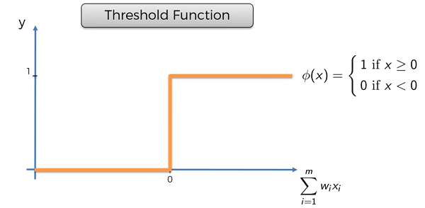
Threshold Function
If the value is less than zero, then the function will pass on zero otherwise it will pass on 1.
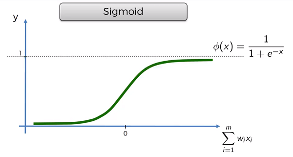
Sigmoid Function
Smooth function, that is especially useful in the output layer for predicting things like probability
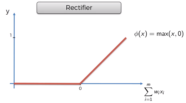
Rectifier Function
The most used function. Usually applied in the hidden layers.
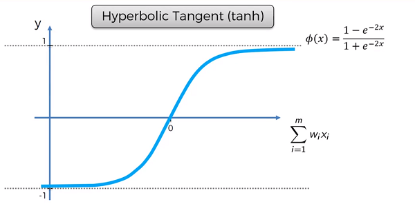
Hyperbolic Tangent Function
More Detail: Deep Sparse Rectifier Neural Networks by Xavier Glorot
How Neural Networks Learn
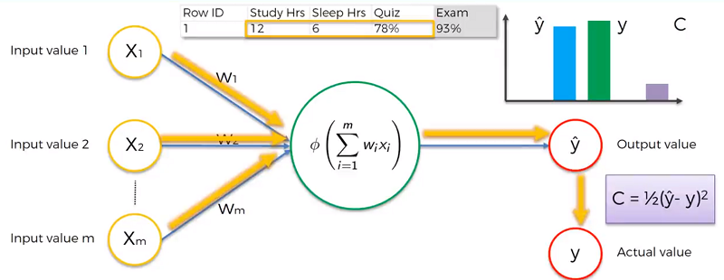
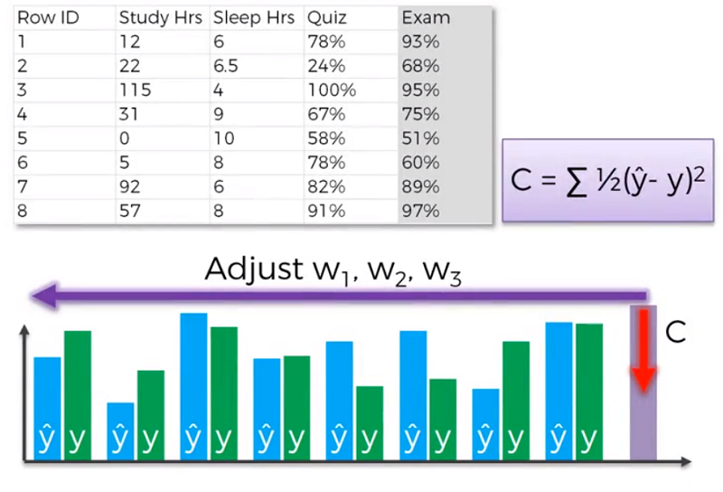
The y hat specifies that it is an output value of the neural net. Y specifies the actual value.
The first step a neural network takes is forward propagation. This is where the inputs will be used by the neuron, an activation function is applied by the neuron an and outvalue is generated. The cost function, C, is then calculated using the outvalue and the actual value.
Back Propagation is sending the cost function back through the network and updating all the weights. This is done until we’ve minimized the cost function. Remember the input values never change, only the weights are affected.
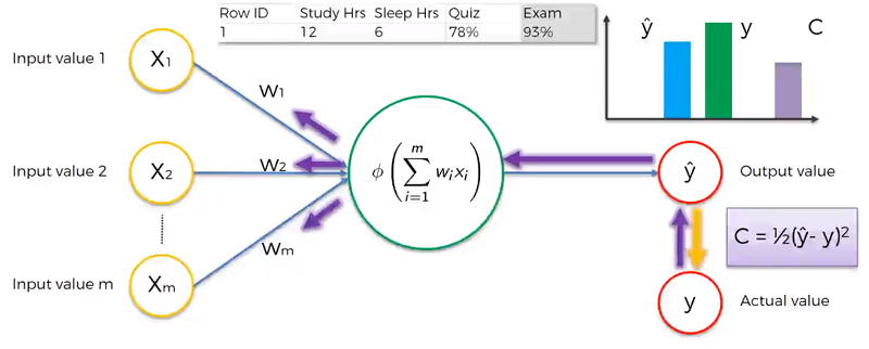
Looking at many lines of data the process would be the following. We would go through each row of the dataset and get the output value. The sum of all the cost functions would be applied and backprop is used on the ANN to adjust the weights. This is done repeatedly for many epochs (an epoch is going through the dataset once).
A list of cost functions used in neural networks alongside applications
Gradient Descent
To minimize the cost function, we use gradient descent (since brute force is far too computationally intensive (Curse of Dimensionality)).
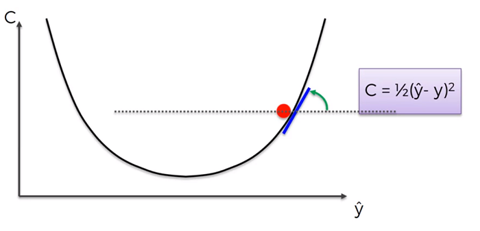
The gradient descant is a method used to find the lowest point on a line (that is convex). The method is simple.
- Start at some point on the curve
- Find the tangent line at that point (if its negative you’re going down the slope and positive means you’re going up the slope).
- The intersection where the tangent line meets the x axis is what we want. That intersection has a corresponding point on the curve.
That point is our new point.
- We do this process until we reach the lowest point. Where the tangent line is 0 (or closest to it).
Stochastic Gradient Descent
When the cost function is not convex, we use stochastic Gradient Descent. Since regular gradient descent may find the local minimum and not the actual minimum of the function.
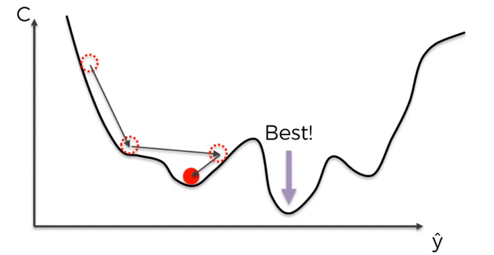
In practice the difference will be that when trying to optimize the cost function, normal gradient descent will use all the rows (or a batch of rows) and apply a weight change based on their sums.
With stochastic gradient descent the weights are adjusted after each row. Stochastic gradient descent is faster than regular gradient decent.
A Neural Network in 13 lines of Python
Neural Networks and Deep Learning
Back Propagation
Step 1: Randomly initialize the weights to small numbers close to 0 (but not 0)
Step 2: Input the first observation of your dataset in the input layer, each feature in one input node.
Step 3: Forward-Propagation: from left to right, the neurons are activated in a way that the impact of each neuron’s activation is limited by the weights. Propagate the activations until the predicted result y.
Step 4: Compare the predicted result to the actual value. Measure the generated error.
Step 5: Back propagating: from left- right, the error is back-propagated. Update the weights according to how much they are responsible for the error. The learning rate decides by how much we update the weights.
Step 6: Repeat Step 1 to 5 and update the weights after each observation (Reinforcement Learning).
Or: Repeat Step 1 to 5 but update the weights only after a batch of observations (Batch Learning).