Introduction
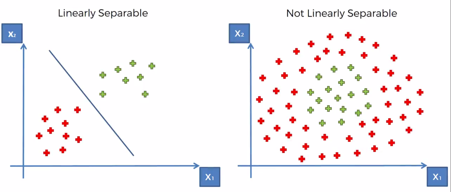
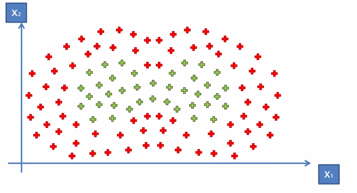
Kernal SVM is used in cases where the dataset is not linearily seperable. This can be seen in the example below where clearlily the dataset is seperable but there is no one line that will be able to do it well.
Mapping in Higher Dimensional Space
The basic concept is simple. We map the dataset to higher dimension, where it is possible to linealiy sepreate the dataset. We then find out seperation, invoke the SVM algorthm to build our discision boundary and then finally return it to our original dimension.
Simple Example of firdt dimension
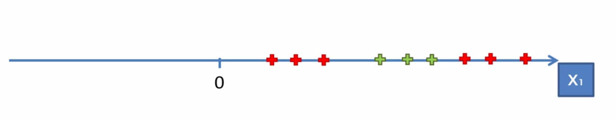
Looking at an example of dataset in the first dimesion we can see that there is no one line (in the case actuallly a dot since it’s one dimensional) to seperate the dataset. So we can apply the method of mapping the dataset onto a higher dimesion to see if there is a way to seperate create discision boundary.
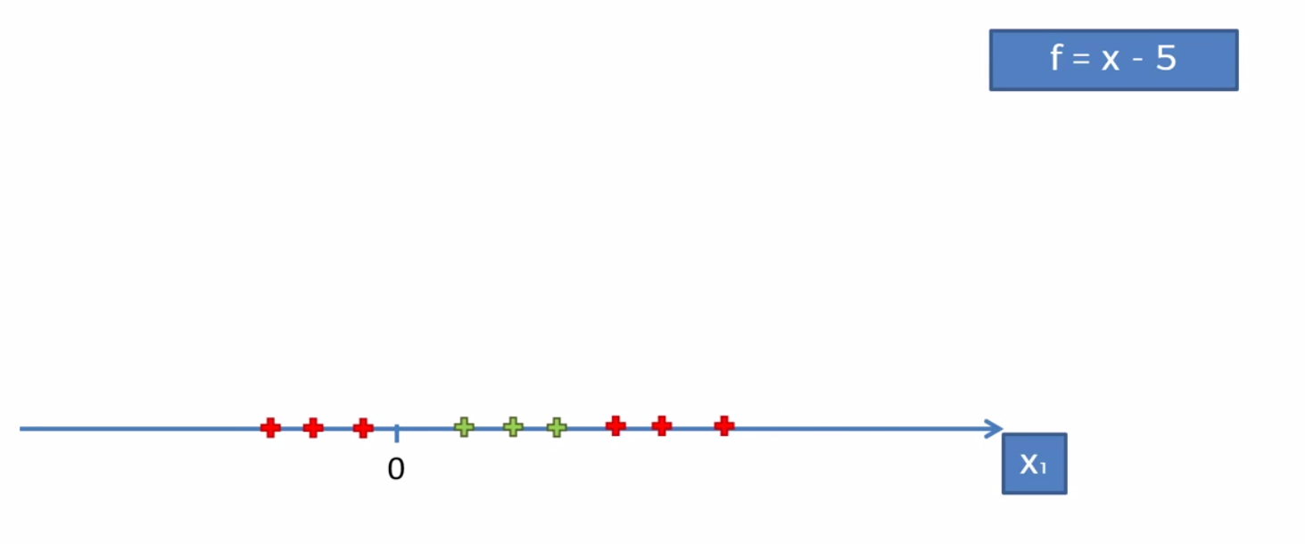
To map the function onto a higher dimesion we’ll need to follow some basic algebraic rules. We can say that the orginal function is F = x. First we want to subtract 5 (in this case). The reason is we want to have some points (namely the red ones) below zero. This will help us making it more seperable when moving to a higher dimension (you’ll need to play with it until it works). We then simple map it on to a parabola (a 2 dimensional line) and voila we can now sepreate the function.
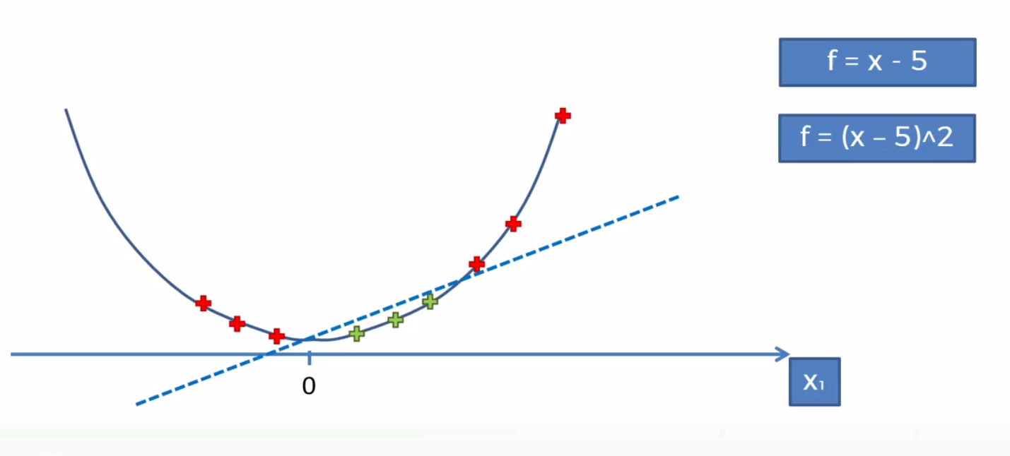
We then would project it back to the 1st dimension and be left with our result.
2nd Dimension the 3rd Dimension
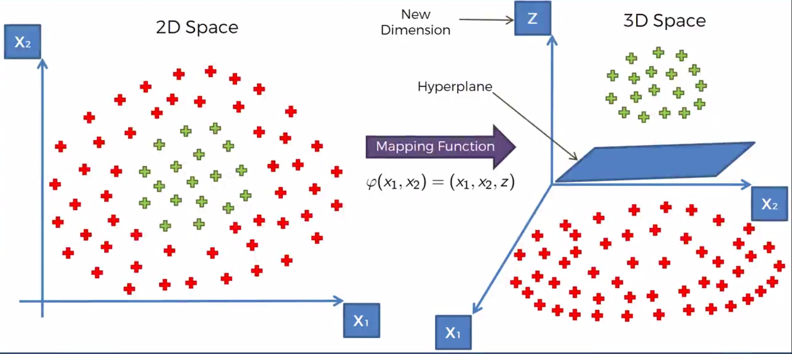
The following visulalization should help in understanding how the mapping works.
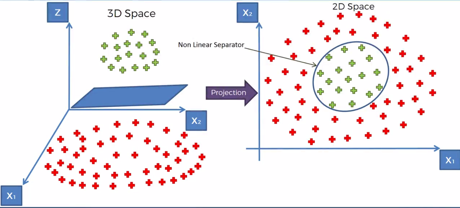
Here we map the points of the dataset from the 2nd dimension to the 3rd. We then using a Hyperplane sepreate the dataset in the manner that we want. Once the dataset is serperated we can project the function back down to the 2nd dimension
Now, we have a disicison boundary created by our SVm ready to be used.
The problem with this approacg is that it is computationally ver intensive and therefore is not a great method when dealing with large sets of data.
The Kernal trick
The Gaussian RBF Kernel
Where,
- : X vector (some point in our dataset)
- : l stands for landmarks (i represents the number of landmarks)
- : Distance between a point and the landmark squared
The landmark is placed directly at the center of the dataset and is used to calculate the distance to a point. In the picture below the landmark is represented by a red dot. The red and green plus signs represent different data points.
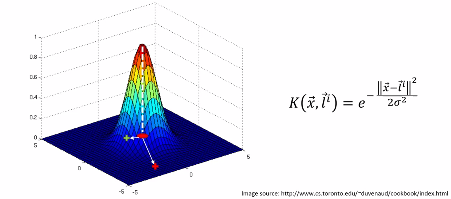
To understand how this function works we’ll walk through it. Looking at the distance between the landmark and the red point we see that the . Squaring this value we get an even larger value. Assuming sigma is large as well the entire exponent is a large value. The negative of a large exponent is a number very close to zero on the y axis. Looking at the point green point on we see that difference is smaller and so the exponent itself will be smaller. The negative of a smaller value will be further from zero generating for us the graph above.
To understand this better, let us look at the the dataset to see how the Gaussian RBF function works.
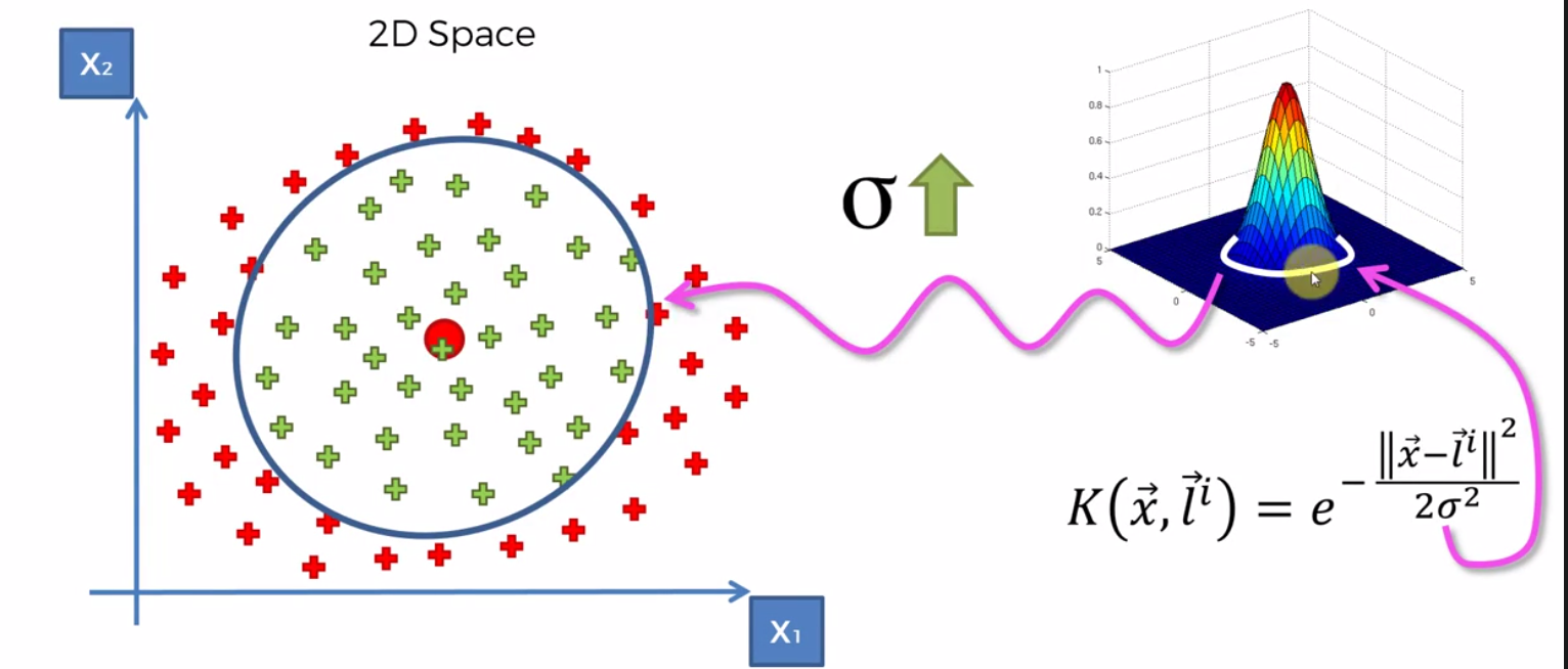
The landmark is placed at the center of the green dataset. Once the landmark is selected a circumference around the dataset is chosen based on the dataset. As sigma increases, the circumference increases and as it decreases so does the circumference. The way it works is put simpply, values outside the circle are given a value 0 (or very close) and values within the circle are given a value above zero.
This concept let’s us solve more complicated dataset. For example, in the dataset below, we can apply two landmarks.
Because of how the Gaussian Equation works, the two landwarks don’t really interfere with each other, given a proper sigma value. So that means we can basically just take two kernal functions and add them up to get our decision boundary.
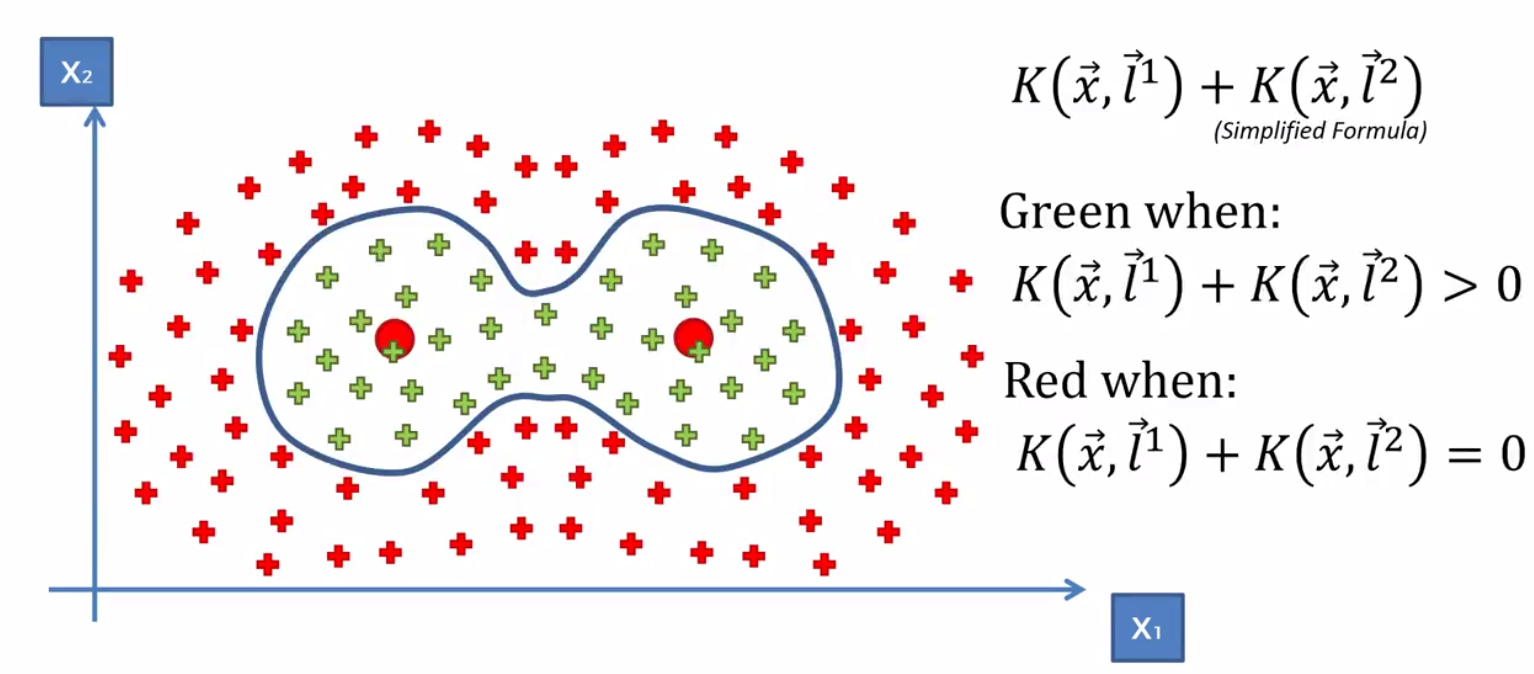
This example however is simplified. In reality we should get the green to be greater or equal to zero and the red is less than zero.
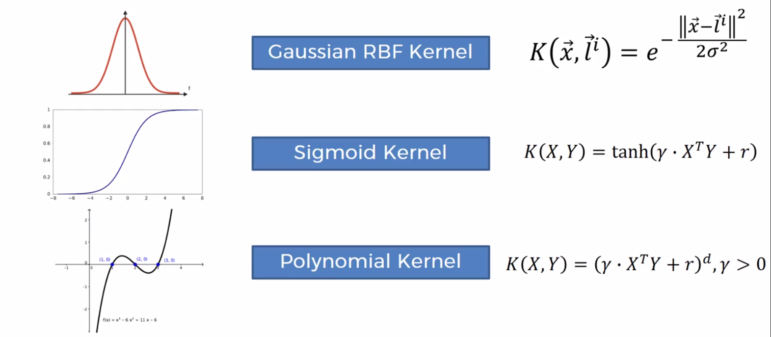
Types of Kernal Functions
Building an SVM (Not linearily seperable)
Create classifer
kernal : linear, poly, rbf
from sklearn.svm import SVC
classifier = SVC(kernel = 'rbf', random_state = 0)
classifier.fit(X_train, y_train)